Top 50 Excel Interview Questions and Answers You Need to Know

Excel is one software that all companies expect you to know and going unprepared for it would be disastrous. Do not worry because here an article dedicated to preparing you for your interviews with the most frequently asked Excel Interview Questions and Answers.

The questions here will be divided into three sections as mentioned below

General Questions:

Q1) Explain MS Excel in brief.

Microsoft Excel is a spreadsheet or a computer application that allows the storage of data in the form of a table. Excel was developed by Microsoft and can be used on various operating systems such as Windows, macOS, IOS and Android.

Excel Interview Questions

Some of the important features of MS Excel are:

• Availability of Graphing tools
• Built-in functions such as SUM, DATE, COUNTIF, etc
• Allows data analysis through tables, charts, filters, etc
• The availability of Visual Basic for Application (VBA)
• Flexible workbook and worksheet operations
• Allows easy data validation

Q2) What do you mean by cells in an Excel sheet?

The area which falls at the intersection of a column and a row where the information is to be inserted is known as a cell. There are a total of 1,048,576 x 16,384 cells present in a single excel sheet.

Excel Interview Questions

Q3) Explain what is a spreadsheet?

Spreadsheets are a collection of cells that help you manage the data. A single workbook may have more than one worksheet. You can see all the sheets at the bottom of the window, along with the names that you have given them. Take a look at the image below:

Q4) What do you mean by cell address?

The cell address of an Excel sheet refers to the address that is obtained by the combination of the Row number and the Column alphabet. Each cell of an MS Excel sheet will have a distinct cell address.

Excel Interview Questions

Q5) Can you add cells?

Yes, you can insert new cells into a sheet. To add a new cell, simply select the cell where you want to insert it and then select the Insert option. you will see the following window:

Select the desired option and then click on OK.

Excel Interview Questions

Q6) Can you format MS Excel cells? If yes, then how?

Yes, MS Excel cells can be formatted. In order to format these cells, you can use the commands present in the Font group of the Home tab. When you open the Font window, you will see the following options:

Name	Description
Number	Allows formatting cells to be of any type such as currency, accounting, date, percentage, etc
Alignment	Allows text control, alignment and setting its direction
Font	Enables various fonts, styles, sizes, colors, etc
Border	Allows cell borders to be changed, removed, colored, etc
Fill	Enables you to choose different colors and styles to fill up the cell
Protection	Allows you to lock or hide cells

Q7) Can you add comments to a cell?

Yes, comments can be added. To add comments to a cell, select the cell, right-click on it and then select the New Comment option. These comments will be visible to all those people who have access to the Excel sheet.

Excel Interview Questions

Q8) Can you add new rows and columns to an Excel sheet?

Yes, you can add rows and columns to an Excel sheet. To add new rows and columns select the place where you intend to add them and right-click on it. Then select the Insert option from where you can choose to select an entire row or column.

Q9) What is Ribbon and where does it appear?

The Ribbon is basically your key interface with Excel and it appears at the top of the Excel window. It allows users to access many of the most important commands directly. It consists of many tabs such as File, Home, View, Insert, etc. You can also customize the ribbon to suit your preferences. To customize the Ribbon, right-click on it and select the “Customize the Ribbon” option. You will see the following window:

You can select or unselect any option of your choice from here.

Q10) How do you freeze panes in Excel?

MS Excel allows you to freeze panes that will help you see the headings of the rows and the columns even if scroll down a long way on the sheet. To Freeze Panes in Excel, follow the given steps:

1. First, select the Rows and Columns you wish to freeze
2. Then, select Freeze Pane present in the View tab
3. Here, you will see the following three options to selectively freeze the rows and columns as shown in the image below:

Q11) How do you add a Note to a cell?

To add a Note, select the cell and right-click on the same. then select the New Note option and type in any note that you wish to. In case you want to delete the Note, follow the same procedure and select the Delete Note option. Notes are indicated by a red triangle at the top-right corner of the cell.

Q12) Can you protect workbooks in Excel?

Yes, workbooks can be protected. Excel provides three options for this:

1. Passwords can be set to open Workbooks
2. You can protect sheets from being added, deleted, hidden or unhidden
3. Protecting window sizes or positions from being changed

Q13) How do you apply a single format to all the sheets present in a workbook?

To apply the same format to all the sheets of a workbook, follow the given steps:

1. Right-click on any sheet present in that workbook
2. Then, click on the Select All Sheets option
3. Format any of the sheets and you will see that the format has been applied to all the other sheets as well

Q14) What do you understand by Relative Cell Addresses?

Whenever you copy formulas in Excel, the addresses of the reference cells get modified automatically in order to match the position where the formula is copied. This is done by a system that is called Relative Cell Addresses.

Excel Interview Questions

EXAMPLE:

Take a look at the image below where I have written the formula in C9 and copying the same formula to C10. As you can see, C10 shows the sum of A10 and B10, unlike A9 and B9.

Q15) In case you don’t want to modify the cell addresses when they are copied, what should you do?

If you do not want Excel to change the addresses when you copy formulas, you must make use of Absolute Cell Addresses. When you use Absolute Cell References, the row and the column addresses do not get modified and remain the same.

Example:

For absolute referencing, you will need to use the $ sign before column and row number. Take a look at the example shown in the given image:

 

 

Q16) What will you do if you want to change either the column letter or the row number but not both?

To do this, you must make use of Mixed Cell Addresses where either the row or column is relative while the other is absolute.

EXAMPLE:

Take a look at the image below where the columns hold relative referencing while the rows are absolute. Therefore, the values that are to be added in C9 are 5 and 5 since the column letter is the same as in the original formula and hence the result.

Q17) Can you protect cells of a sheet from being copied?

Yes, you can do it by protecting the required cells or the complete sheet. In order to do this, follow the given steps:

1. Select the cells that you want to protect
2. Open up the Font window from the Home tab
3. From the Protection pane, select Protection and then check the Hidden box
4. Click on Review tab present in the Ribbon, and then select Protect sheet option (Excel will not hide the required cells unless you do this)
5. Specify a password (This will help you in unprotecting the sheet later)

Q18) How do you create Named Ranges?

To create named ranges, follow the given steps:

• Select the area to which you intend to give a name
• From Ribbon, select Formulas
• Click on Define Name from Defined Names group
• Give any name of your choice

Q19) What are macros?

Excel allows you to automate the tasks you do regularly by recording them into macros. So, a macro is an action or a set of them that you can perform n number of times. For example, if you have to record the sales of each item at the end of the day, you can create a macro that will automatically calculate the sales, profits, loss, etc and use the same for the future instead of manually calculating it every day.

Q20) How do you create dropdown lists in Excel?

To create dropdown lists, follow the given steps:

• Click on Data tab present in the ribbon
• Then, from the Data Tools group, click on Data Validation
• Navigate to Settings>Allow>List
• Select the source list array

Pivot Tables and Pivot charts:

Q21) Explain Pivot tables along with their features?

Pivot Tables are statistical tables that condense data of those tables that have extensive information. The summary can be based on any field such as sales, averages, sums, etc that the pivot table represents in a simple and intelligent manner.

Features:

Some of the features of Excel Pivot Tables are as follows:

• Allow the display of exact data you have to analyze
• Provide various angles to view the data
• Allow you to focus on important details
• Comparison of data is very handy
• Pivot tables can detect different patterns, relationships, data trends, etc
• They can create instant data
• Accurate reports
• Serve the base for Pivot charts

Q22) How do you create Pivot Tables?

In order to create a Pivot table, you will first need to prepare the data in a tabular format. Keep the following points in mind while preparing the data:

• Arrange the data into rows and columns
• The first row should contain unique heading for each of the columns
• The columns should have only one type of data
• Rows must have data for a single recording only
• No blank rows
• Columns should not be completely blank
• The data for creating Pivot table should be separate from other data present in the sheet

For example, let’s create a Pivot chart for the table shown in the image below:

To create a Pivot table, select the table and click on the Insert tab. then select Pivot Table command  and you will see the following window:

Specify where you intend to create the table and then click on OK. Once this is done you will see that an empty pivot table has been created. Also, PivotTables Fields pane will open that will help you configure the Pivot table. Take a look at the image below where I have created a Pivot Table:

Q23) What are Pivot charts in MS Excel?

MS Excel charts are data visualization tools that help you visualize data in various ways. These charts can be of any type such as Bar, Pie, Area, Line, Doughnut, etc. For example, take a look at the Pivot table in the image below:

Now, if you wish to create a pivot chart for this table, select any cell from the table and then from the Insert tab, choose the Pivot Chart option. You will see the following options:

Choose any chart of your preference and click on OK. You can also format these charts respectively.

Q24) Can you create Pivot tables using multiple tables?

Yes, you can create Pivot tables using more than one base table. To do this, follow the given steps:

1. Press Alt+D and then press P to open up the PivotTable Wizard
2. Then select Multiple consolidation ranges option and click on Next and you will see another dialog box as shown below:
3. Select I will create the page fields option and click on Next
4. In the next window, you will need to add all the required ranges as shown below:
5. Once that is done, click on Next
6. Specify the region where you want to create the table and then click on Finish
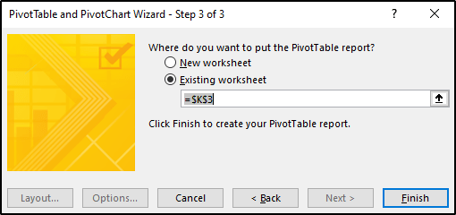
7. You will see the pivot table has been created by merging both the tables as shown in the image below:

Q25) What happens when you check the Defer Layout Update option present in the PivotTable Fields window?

In case you check this option, you will not see dynamic changes while interchanging the table fields. By default, this option is off or unchecked.  All the changes will appear only after you click on the Update button when you check this box.

Q26) Can you create a pivot table using tables from different worksheets?

If both the sheets are from the same workbook, you can create a pivot table for tables from different sheets as well. To create a pivot table from two different sheets, follow the same steps as shown in Q24 and when you specify the tables, go to the respective sheet and select the tables you intend to merge.

Q27) Is it possible to see the details of the results displayed in a pivot table?

Yes, it is possible to see the details of the results shown by the pivot tables in Excel. In order to see the details for any result, double-click on the value and you will see that a new sheet has been created with a new table having details about the factors that have led to that particular result. For example, if I double-click on one of the city values for Brad in the pivot table shown in Q15, I will see the following table that displays the details regarding the same:

Q28) How are PivotTables used to filter data?

Excel PivotTables allow you to filter data according to your requirements. To do this, place the field based on which you wish to filter out the data. Then from the pivot table, open the dropdown list present for the field you have placed in the Filter area and select the section of your choice. For example, in the table shown in Q22, if you wish to filter the data for different cities, you can do it easily as shown below:

As you can see, I have filtered the data for Chicago.

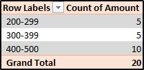
Q29) How do you change the value field to show some other result other than the Sum?

In order to change the value field to show results other than the Sum, right-click on the Sum of Amount values and then click on Value Field Settings. Here is the dialog box that you will see:

From here, you can select any value of your choice and then click on OK.

Q30) How to stop automatic sorting in PivotTables?

Excel automatically sorts the data present in the Pivot Tables. In case you do not want Excel to do this, open the dropdown menu fro the Row Labels or the Column Labels, and then click on More Sort Options. You will see the Sort dialog box opening. Click on More Options and unselect the Sort automatically option.

Excel Interview Questions

Formulas and Functions:

Q31) What do you understand by Excel functions?

Functions, in Excel, are used to perform specific tasks. Excel has many built-in functions that are used to calculate results of various formulas thereby helping in time conservation. Also, these functions make it very easy to execute formulas which would have been difficult to manually write down.

Excel Interview Questions

Q32) What are the various categories of functions available in Excel?

Functions in Excel are categorized as follows:

Catagory	Important Formulas
Date & Time	DAY, DATE, MONTH, etc
Financial	ACCINTM, DOLLARDE, ACCINT, etc
Math & Trig	SUM, SUMIF, PRODUCT, SIN, COS, etc
Statistical	AVERAGE, COUNT, COUNTIF, MAX, MIN, etc
Lookup & Reference	COLUMN, HLOOKUP, ROW, VLOOKUP, CHOOSE, etc
Database	DAVERAGE, DCOUNT, DMIN, DMAX, etc
Text	BAHTTEXT, DOLLAR, LOWER, UPPER, etc
Logical	AND, OR, NOT, IF, TRUE, FALSE, etc
Information	INFO, ERROR.TYPE, TYPE, ISERROR, etc
Engineering	COMPLEX, CONVERT, DELTA, OCT2BIN, etc
Cube	CUBESET, CUBENUMBER, CUBEVALUE, etc
Compatibility	PERCENTILE, RANK, VAR, MODE, etc
Web	ENCODEURL, FILTERXML, WEBSERVICE

Q33) What is the operator precedence of formulas in Excel?

Formulas in Excel are executed according to the BODMAS rules. BODMAS, as many of us know, stands for Brackets Order Division Multiplication Addition and Subtraction. That means, in every formula, brackets are executed first (if they are present) followed by multiplication, division, etc. An example of the same is shown in the image below:

As you can see, the output is 27 i.e obtained by first adding 4+5 and then multiplying it by 3. In case you do not specify the brackets, you will get the result by first multiplying 3×4 and then adding 5 to it i.e 12+5 resulting in 17.

Q34) Explain SUM and SUMIF functions.

SUM: The SUM function is used to calculate the sum of all the values that are specified as a parameter to it. The syntax of this function is as follows:

SUM(number1, number2, …)

EXAMPLE:

As you can see in the image, the SUM function is calculating the total price for all the vegetables.

SUMIF: This function is used to calculate the sum of values that comply with a given condition.

SYNTAX:

SUMIF(range, criteria, [sum_range])

where,

• range specifies the range of cells to be evaluated
• criteria provides the condition to be met
• sum_range is optional and provides the actual cells to be summed up

EXAMPLE:

As you can see, the SUMIF function is calculating the sum of goals scored only by Dybala.

Q35) What are the different types of COUNT functions available in Excel?

Excel provides five types of COUNT functions i.e COUNT, COUNTA, COUNTBLANK, COUNTIF, and COUNTIFS.

The COUNT returns the total number of cells that have numbers in the range that is specified to it as a parameter.

SYNTAX:

COUNT(value1, value2, …)

EXAMPLE:

 

In the above image, you can see that the COUNT function is used to calculate the number of cells having numerical data in them.

COUNTA: Counts the number of cells in a given range that are not empty.

SYNTAX:

COUNT(value1, [value2], …)

EXAMPLE:

The above image shows the functionality of the COUNTA function that returns the number of cells that are not between A4 and B10.

COUNTIF: This function counts the number of cells that comply to a given condition.

SYNTAX:

COUNTIF(range, criteria)

EXAMPLE:

Take a look at the image below, where the COUNTIF function is used to calculate the number of cells that have the name, Dybala.

 

COUNTBLANK: Counts all the blank cells in a given range.

SYNTAX:

COUNTBLANK(range)

EXAMPLE:

COUNTIFS: This is a special function that allows you to specify a set of conditions in order to count them.

SYNTAX:

COUNTIFS(criteria_range1,range1,[criteria_range2, criteria2], …)

EXAMPLE:

Q36) How do you calculate the percentage in Excel?

Percentages, as we all know, are ratios that are calculated as a fraction of 100. Mathematically, the percentage can be defined as follows:

Percentage = (Part/ Whole) x 100

In Excel, the percentage can be calculated in a similar manner. Take a look at the image below where the percentage has been calculated for the values present in A1 and A2.

Here are the steps followed in order to obtain the result:

• Select the cell destination cell to display the percentage
• Then, type a “=” sign
• Type in A1/ A2 then hit the Enter key
• Click on Home tab, select % symbol from the numbers group

Q37) Explain how to calculate compound interest in Excel?

To calculate compound interest in Excel, you can use the FV function. FV returns the future value of an investment based on the periodic, constant interest rate and payments.

SYNTAX:

FV(rate, nper, pmt, pv, type)

To find the rate, the number of periods are used to divide the annual rate (annual rate/ periods). nper is obtained by multiplying the no. of years (term) with the periods (term * periods). Periodic payment (pmt) can be any value (including zero).

EXAMPLE:

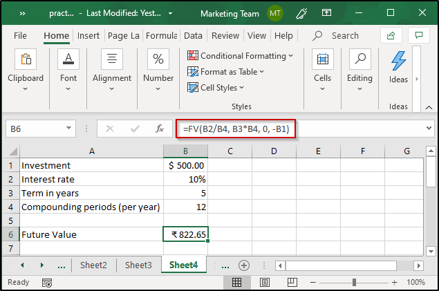
The investment amount is $500, rate is 10% for 5 years. There are no periodic payments hence the value for pmt is 0. -B1 means that $500 has been taken from you. Therefore, the FV for this is $822.65.

Q38) How do you find averages in MS Excel?

Average can be calculated using the AVERAGE function.

SYNTAX:

AVERAGE(number1, number2, …)

EXAMPLE:

 

To calculate the average marks scored by Dave and Ava, I have used the AVERAGE function.

Q39) What is VLOOKUP in Excel?

VLOOKUP is a function present in Excel used to lookup and bring forth data from a given range. V in VLOOKUP stands for Vertical and to use this function, data should be arranged vertically. VLOOKUP is very useful when you have to find some piece of data from a huge amount of data.

Q40) How does the VLOOKUP function work?

The VLOOKUP function, in Excel, a lookup value and begins to look for the same in the leftmost column. When it finds the first occurrence of the given lookup value, VLOOKUP starts to move right i.e in the row where the value was found. It goes on until the column number specified by the user and returns the desired value. This function is used to match exact and approximate lookup values. However, the default match is an approximate match.

Syntax:

VLOOKUP(lookup_value, table_array, col_index_num, [range_lookup])

here,

• lookup_value gives the value to be looked out for
• table_index is the range from where the data is to be taken
• col_index_num specifies the column from which you want to fetch the value
• range_lookup is a logical value i.e TRUE or FALSE (TRUE will find the closest match; FALSE checks for exact match)

Q41) Explain the exact match with an example.

For an exact match, set the range_lookup value as FALSE.

EXAMPLE:

In case you want to look for the designation of an employee, follow the given steps:

• Select the destination cell and type “=”
• Use VLOOKUP
• Specify the lookup_value (Here, it is the ID) along with the other parameters
• Set range_lookup value to FALSE
• The function will be: =VLOOKUP(104, A1: D8, 3, FALSE)

As you can see, VLOOKUP has returned the designation of the employee having 104 as his ID.

Q42) Explain the approximate match with an example.

For an approximate match, VLOOKUP will fetch values when there are no exact matches of the given loopup_value. For an approximate match, set the range_lookup value to TRUE. Remember that the table must be sorted in ascending order for VLOOKUP to do an approximate match. So here, VLOOKUP basically starts to look for an approximate match of the given lookup value and the, stops at a value that is next largest of the given lookup value. It then moves into that row to return the value from the column that has been specified.

The following image shows an example of an approximate match by VLOOKUP:

 

• Follow the same steps specified for exact match
• For the range_lookup value, use TRUE
• The function will be: =VLOOKUP(55, A12: C15, 3, TRUE)

The lookup value is 55 and the next largest of the lookup value present in the first column is 40. Hence, the output is ‘Second Class’.

Q43) Can you use VLOOKUP for multiple tables?

Yes, you can use VLOOKUP for multiple tables as well.  In case you have two lookup tables, create named ranges for each table, and then use the IF function to select between each table based on some given condition. Click here to know more about this.

Q44) How do you perform a horizontal lookup in Excel?

To perform a horizontal lookup, you will have to make use of the HLOOKUP function.

SYNTAX:

HLOOKUP(lookup_value, table_array, row_index_num, [range_lookup])

here,

• lookup_value gives the value to be looked out for
• table_index is the range from where the data is to be taken
• row_index_num specifies the row from which you want to fetch the value
• range_lookup is a logical value i.e TRUE or FALSE (TRUE will find the closest match; FALSE checks for exact match)

EXAMPLE:

Q45) How will you fetch the current date in Excel?

You can make use of the TODAY function. This function will return the current date in the MS Excel date format.

SYNTAX:

TODAY()

EXAMPLE:

 

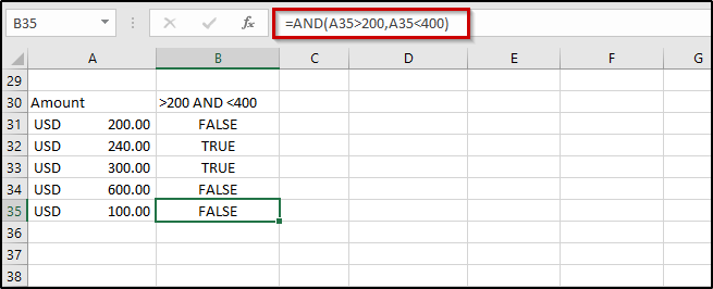
Q46) How does the AND function work?

The AND function in Excel is used to whether a given condition or a set of conditions is TRUE or not. In case all the conditions are satisfied, this function will return a boolean TRUE.

SYNTAX:

AND(logical1, [logical2], …)

where,

logical1, logical2, … are conditions from 1-255 that you want to check

EXAMPLE:

Q47) What is the What If Analysis?

What If Analysis is the technique of performing changes to one or more formulas present in the cells in order to see how it affects the result of those formulas in the worksheet. Excel provides three types of What If Analysis tools:

1. Scenarios
2. Goal Seek
3. Data Tables

Scenarios and Data Tables take a set of inputs to check for the potential results. Scenarios can work with many variables but input values can be at the max 32. Data tables, on the other hand, work with just one or two variables but can accept many distinct values for each of those variables.

Excel Interview Questions

Goal Seek, in contrast to Scenarios and Data Tables, takes the outputs and determines the possible inputs for the same.

Q48) Can you create shortcuts for most frequently used formulas?

Yes, you can do it by customizing the Quick Access Toolbar. To customize it, right-click anywhere on the Quick Access Toolbar and select the Customize Quick Access Toolbar option. You will see the following window:

From here, select Formulas and then choose any formula that you wish to create a shortcut for.

Excel Interview Questions

Q49) What is the difference between formulas and functions in Excel?

Formulas are that are defined by the user that is used to calculate some results. Formulas either be simple or complex and they can consist of values, functions, defined names, etc.

A function, on the other hand, is a built-in piece of code that is used to perform some particular action. Excel provides a huge number of built-in functions such as SUM, PRODUCT, IF, SUMIF, COUNT, etc.

Q50) How do you use wildcards with VLOOKUP?

Wildcards can be used when you are not sure of the exact lookup value. In order to use wildcards in Excel, you should make use of the “*” symbol.

Excel Interview Questions

For example, in the table that you see in the image below, if you enter “erg” and then use wildcards with it, VLOOKUP will fetch the output that corresponds to “Sergio”.